Overview

This article is an introduction to CockroachDB archival partitioning, which is a form of table partitioning that allows storing infrequently-accessed data on specific nodes in a cluster with slower and cheaper storage.

Archival Use Cases

CockroachDB is crafted to provide strong consistency with high scalability, performance and fault-tolerance for OLTP workloads across all parts of the keyspace. For optimal performance it's recommend to use local SSDs or NVMe storage.

For high data volumes, it’s quite common to only access low figures of the entire keyspace while the rest just "sits around" for compliance reasons, much like the Pareto distribution principle. This is typically where data archiving solutions comes into play. The purpose of archival strategies is to move infrequently accesed, long-tail data to a separate storage in order to offload the primary database. In CockroachDB however, the long tail data is not necessarily moved off the cluster, but more relocated to nodes with a different hardware profile to reduce cost over time.

Archival in general is the process of moving long tail data to potentially separate and offline storage, but in CockroachDB it can still be online. This can be useful to support certain type of business operations with a long retention period, for example payment or deposit reversals.

Introduction to Partitioning

Manual table partitioning in CockroachDB can be applied in two different ways:

• List / Geo-partitioning allows storing user data close to the proximity of access, which reduces the distance that the data needs to travel, thereby reducing latency.
• Range / Archival-partitioning allows storing infrequently-accessed data on slower and cheaper storage, thereby reducing costs.

List partitioning is a good fit for geographic distribution where the partition keys are fairly small in numbers (like country codes, regions or jurisdictions). List partitioning gives control of both leaseholder and replica placement, which in turn gives predictable read and write performance and the ability to pin data at row level.

Range or archival partitioning on the other hand is a good fit for moving long tail “cold” data ranges to slower/cheaper hardware for archival, based on some timestamp, date range or other interval criteria. For example, automatically moving financial payment transactions older than 90 days to archival-type of database nodes using slower, but bigger disks or even shared storage.

The most common method is list partitioning, which is semantically equivalent to the automated mechanisms used to provide CockroachDB's multi-region capabilities. These are declarative in nature and automatically handle geo-partitioning and other low-level details. It's more or less just about definiting the survival goal for a database:

ALTER DATABASE <db> SURVIVE REGION FAILURE;

This post is however referring to the "manual" approach of defining table partitions, which is most relevant for archival use cases.

Archival Partitioning Example

Let's take a simple example. Here's a simple payments table with a booking_date column being part of the composite primary index:

CREATE TABLE payments
(
    id UUID NOT NULL DEFAULT gen_random_uuid(),
    booking_date DATE,
    reference STRING,
    amount DECIMAL NOT NULL,
    currency STRING NOT NULL,
    archived BOOL NOT NULL DEFAULT false,

    PRIMARY KEY (booking_date, id)
);

Now, let’s use the range partitioning syntax to qualify payment transaction for archival:

ALTER TABLE payments PARTITION BY RANGE (booking_date) (
    PARTITION archived VALUES FROM (MINVALUE) TO ('2022-06-01'),
    PARTITION recent VALUES FROM ('2022-06-01') TO (MAXVALUE)
);

Assuming we set the --store attribute when starting the nodes and labeling the type of storage on each node:

--store=path=/mnt/ssd01,attrs=ssd
--store=path=/mnt/hda1,attrs=hdd

Start command examples, for illustration:

n1: --insecure --background --locality=region=europe-west1,datacenter=europe-west1a --store=path=datafiles/n1,size=15%,attrs=ssd --listen-addr=192.168.2.1:26257 --http-addr=192.168.2.1:7071 --join=192.168.2.1:26257
n2: --insecure --background --locality=region=europe-west1,datacenter=europe-west1b --store=path=datafiles/n2,size=15%,attrs=ssd --listen-addr=192.168.2.1:26258 --http-addr=192.168.2.1:7072 --join=192.168.2.1:26257
n3: --insecure --background --locality=region=europe-west1,datacenter=europe-west1c --store=path=datafiles/n3,size=15%,attrs=ssd --listen-addr=192.168.2.1:26259 --http-addr=192.168.2.1:7073 --join=192.168.2.1:26257
n4: --insecure --background --locality=region=europe-west2,datacenter=europe-west2b --store=path=datafiles/n4,size=15%,attrs=hdd --listen-addr=192.168.2.1:26260 --http-addr=192.168.2.1:7074 --join=192.168.2.1:26257
n5: --insecure --background --locality=region=europe-west3,datacenter=europe-west3a --store=path=datafiles/n5,size=15%,attrs=hdd --listen-addr=192.168.2.1:26261 --http-addr=192.168.2.1:7075 --join=192.168.2.1:26257
n6: --insecure --background --locality=region=europe-west3,datacenter=europe-west3a --store=path=datafiles/n6,size=15%,attrs=hdd --listen-addr=192.168.2.1:26262 --http-addr=192.168.2.1:7076 --join=192.168.2.1:26257

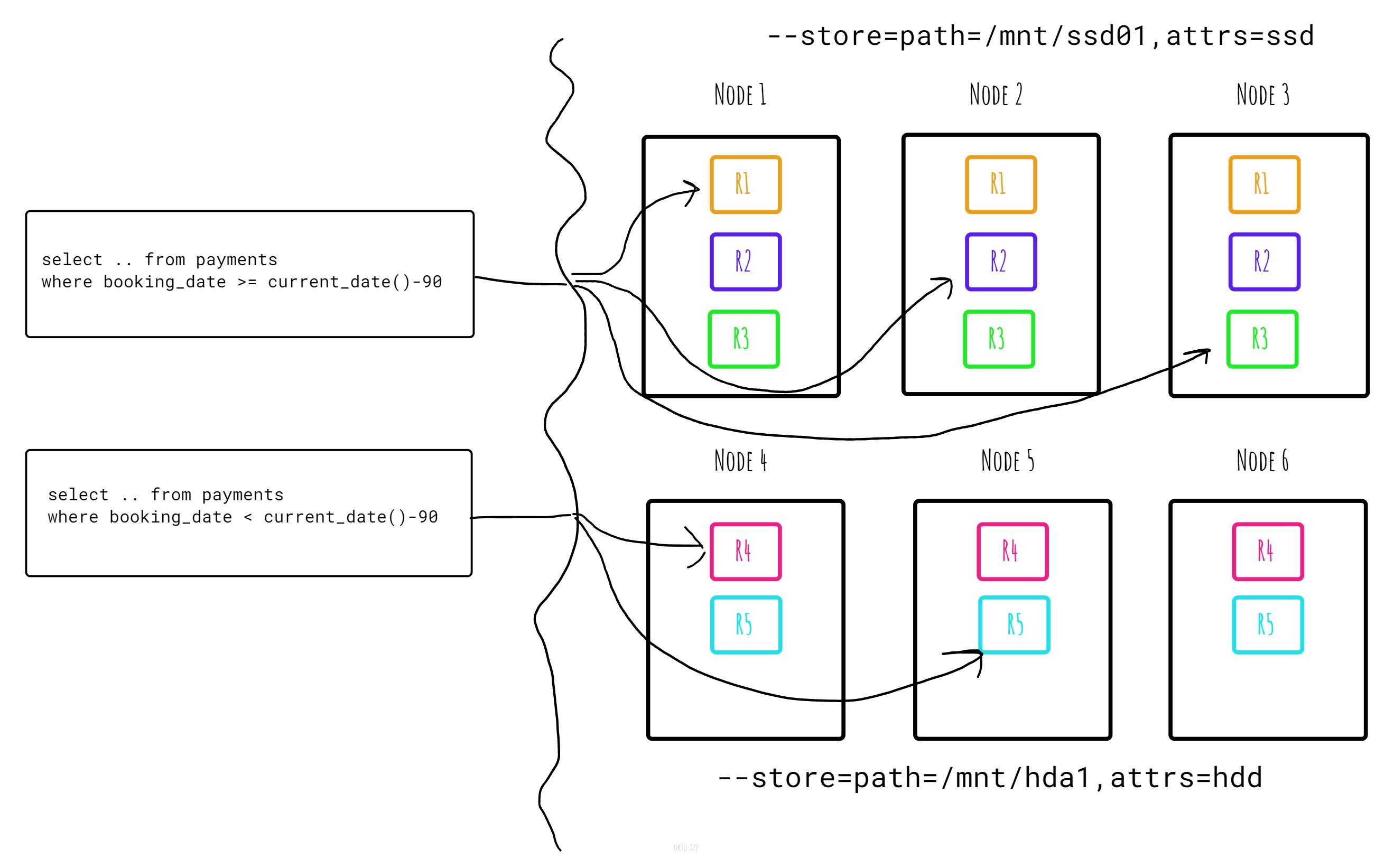
Now we can easily pin each partition of the table matching the given store constraints, ensuring that range replicas holding payments older than 2022-06-01 get stored on nodes with hdd’s, otherwise ssd’s:

ALTER PARTITION recent OF TABLE payments CONFIGURE ZONE USING constraints='[+ssd]';
ALTER PARTITION archived OF TABLE payments CONFIGURE ZONE USING constraints='[+hdd]';

Notice that these attributes are just arbitrary tags or labels, you could use any name really.

Let's verify the range distribution:

SHOW RANGES FROM TABLE payments;

You should see something to the effect of:

start_key | end_key | range_id | range_size_mb | lease_holder |            lease_holder_locality             | replicas |                                                               replica_localities
------------+---------+----------+---------------+--------------+----------------------------------------------+----------+-------------------------------------------------------------------------------------------------------------------------------------------------
  NULL      | NULL    |       85 |             0 |            3 | region=europe-west1,datacenter=europe-west1b | {3,4,6}  | {"region=europe-west1,datacenter=europe-west1b","region=europe-west2,datacenter=europe-west2b","region=europe-west3,datacenter=europe-west3a"}
(1 row)

Now let's configure the zones and apply them to the corresponding partitions. This is when the actual rebalancing take effect:

ALTER PARTITION recent OF TABLE payments CONFIGURE ZONE USING constraints='[+ssd]';
ALTER PARTITION archived OF TABLE payments  CONFIGURE ZONE USING constraints='[+hdd]';

Let's verify the range distribution again:

SHOW RANGES FROM TABLE payments;

You should now see something like this:

start_key | end_key | range_id | range_size_mb | lease_holder |            lease_holder_locality             | replicas |                                                               replica_localities
------------+---------+----------+---------------+--------------+----------------------------------------------+----------+-------------------------------------------------------------------------------------------------------------------------------------------------
  NULL      | /19144  |       70 |             0 |            5 | region=europe-west3,datacenter=europe-west3a | {4,5,6}  | {"region=europe-west2,datacenter=europe-west2b","region=europe-west3,datacenter=europe-west3a","region=europe-west3,datacenter=europe-west3a"}
  /19144    | NULL    |       71 |             0 |            3 | region=europe-west1,datacenter=europe-west1b | {1,2,3}  | {"region=europe-west1,datacenter=europe-west1a","region=europe-west1,datacenter=europe-west1c","region=europe-west1,datacenter=europe-west1b"}
(2 rows)

Lets insert some data to the table to see how things get placed:

INSERT INTO payments(booking_date,reference,amount,currency,archived)
SELECT
    current_date()-170,
    md5(random()::text),
    (no::FLOAT * random())::decimal,
    'SEK',
    false
FROM generate_series(1,100) no;

So here we added payments which are old enough to sort into the archived partition. Let's add a similar volume that is more recent also:

INSERT INTO payments(booking_date,reference,amount,currency,archived)
SELECT
    current_date(),
    md5(random()::text),
    (no::FLOAT * random())::decimal,
    'SEK',
    false
FROM generate_series(1,150) no;

There should be 250 payments in total:

select count(1) from payments where booking_date < '2022-06-01'; -- 100
select count(1) from payments where booking_date >= '2022-06-01'; -- 150

Last by not least, how do we tell where each payment row is stored? We can use SHOW RANGE FROM TABLE which asks the database where it would store a given key, but not that the row actually exist. First lets find a row we know exist:

select booking_date, id from payments where booking_date < '2022-06-01' limit 1;

Now lets find the range for that composite primary key:

select replicas,replica_localities from [                                                                                       SHOW RANGE FROM TABLE payments FOR ROW ('2022-05-14'::date,'078678a4-2448-4189-8e78-0968544bf3da'::uuid)];
  replicas |                                                               replica_localities
-----------+-------------------------------------------------------------------------------------------------------------------------------------------------
  {4,5,6}  | {"region=europe-west2,datacenter=europe-west2b","region=europe-west3,datacenter=europe-west3a","region=europe-west3,datacenter=europe-west3a"}
(1 row)

Now we can confirm the row key is stored in range replicas on nodes 4,5,6 which if you recall happens to be the nodes with [+hdd] locality attributes.

Let's run the same thing for the more recent payements:

select booking_date, id from payments where booking_date >= '2022-06-01' limit 1;

and:

select replicas,replica_localities from [                                                                                       SHOW RANGE FROM TABLE payments FOR ROW ('2022-10-31'::date,'00071e6b-cc7d-4217-ac92-2a7f5a3cb923'::uuid)];
  replicas |                                                               replica_localities
-----------+-------------------------------------------------------------------------------------------------------------------------------------------------
  {1,2,3}  | {"region=europe-west1,datacenter=europe-west1a","region=europe-west1,datacenter=europe-west1c","region=europe-west1,datacenter=europe-west1b"}
(1 row)

Now we have verified that this row key both exist and is stored in range replicas on nodes 1,2,3 which have the [+ssd] locality attribute.

Archival Solution

Eventually you may also want to move long tail range partitioned data to a separate, off-line cloud storage or similar and then purge or delete the source from the online transactional database. CockroachDB doesn’t currently support dropping data associated with partitions (only the configs, in which case data gets rebalanced again). There are still methods to achieve a similar outcome.

One approach is to create a changefeed to a cloud storage sink (or use Kafka or a webhook to bridge between) and then issue an UPDATE to tables with rows to be permanently archived.

UPDATE payments SET archived=true WHERE booking_date < '2022-06-01' and not archived                                        
RETURNING id;

This will return a list of payments marked for archiveal. In addition the update will emit a group of change events (CDC) describing each to-be-deleted row in either JSON or Avro format. There's an option to include the values in the change stream which means no information is lost in the archival store.

After that, the next step is to issue DELETE statements in batches for the archived rows using a predicate to filter out the rows that've been streamed to a downstream cloud storage.

DELETE FROM payments WHERE archived=true;

You would want do some checkpointing before to ensure that all rows have been sent to the downstream sink before deleting.

This type of archival cycle could be built into a shared domain-agnostic service, or become a per-service responsiblity. Data could also be deleded using Row-Level TTL.

Conclusion

We looked at CockroachDB's archival partitioning mechansim to move cold data to nodes with different locality attributes transparently. This can be part of an archival strategy to ultimately remove data after staging in nodes provisioned with more inexpensive storage.