This post will explore a few shortest path search algorithms called Dijkstra's, A* (a-star search) and Bellman-Ford, and how these are leveraged in computer games and other domains.

Example Code

A working demo application for visualising different shortest path search algorithms is available in Github.

Introduction

Finding the shortest path between nodes in a graph is a classical problem solving area in graph theory and computer science. Graphs can be used to model many problem domains. From solving mazes, navigating road networks, packet routing over internet, satellite navigation systems and autonomous robot guidance.

In computer gaming, graphs are often used as a backbone for designing AI behaviour around path finding.

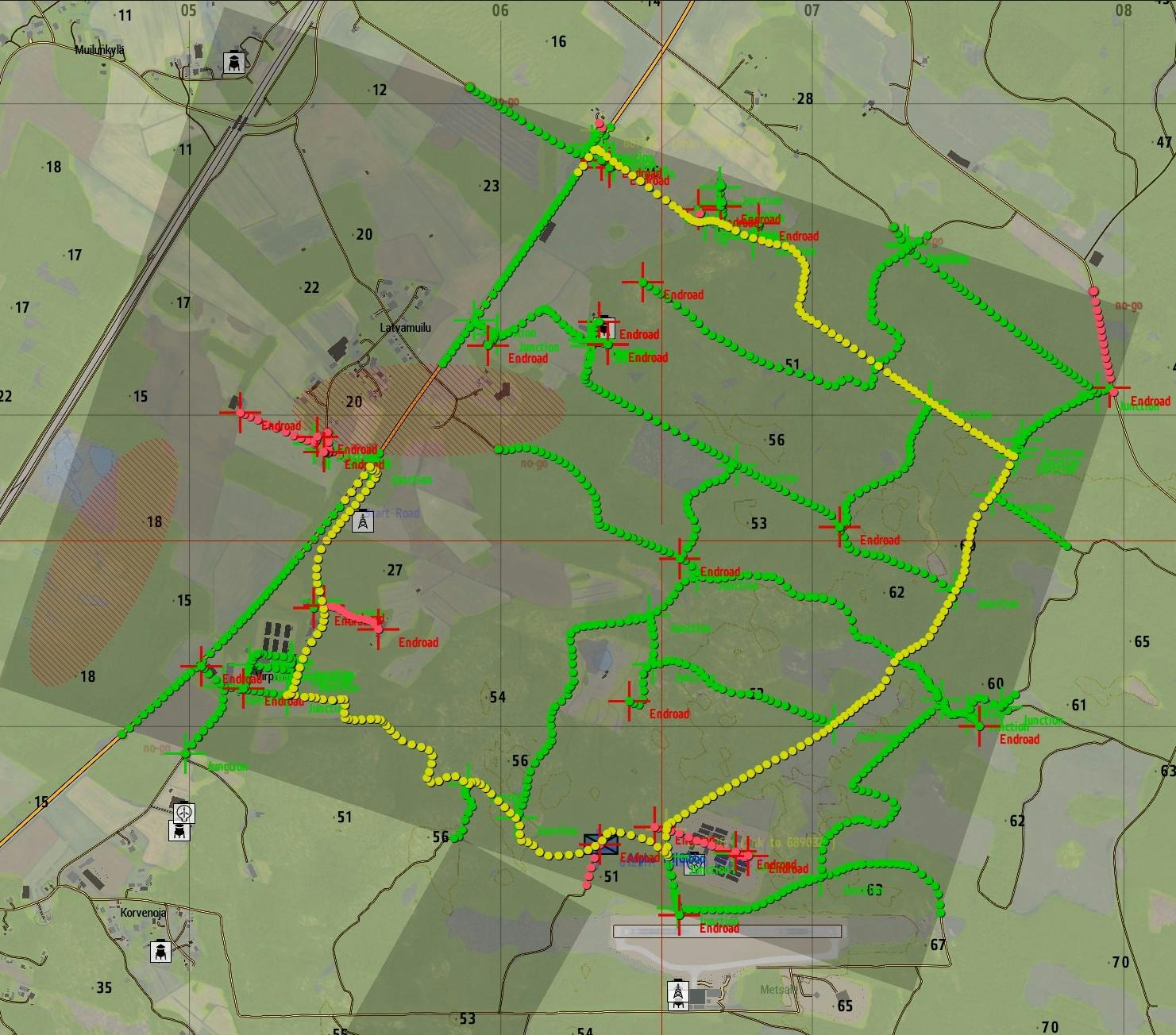
Imagine an AI controlled unit or squad that needs to move between point A and B in a terrain model concealed without confrontation. That could be done both foot mobile or mounted on a vehicle leading to different paths depending on combat mode, avoiding obstacles, fortifications and strongholds where there's exposure to enemy fire.

Between the start and target positions, there can be a road network of smaller dirt roads, paved highways and country roads. There are also bridges and towns, minefields and fortified positions that are considered risky or no-go zones.

Finding the optimal path across that network to a destination needs to use some kind of lowest-cost path finding intelligence. Let's enter the world of shortest path search algorithms.

(Image from Arma3)

Graph Theory Primer

A graph is a mathematical structure with nodes (vertices) and edges (arcs) that connect nodes together. In a road map, a node is a city and an edge is the road connecting two cities. A directed edge is a one-way road, and undirected is a two-way road.

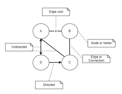
Nodes can be interconnected in many different ways which also determines if the graph is directed, undirected, cyclic or acyclic.

• A directed graph have edges that go in one direction but not the other.
• An undirected graph have edges that go in both directions.
• A cyclic graph have nodes forming a closed cycle where a node is reachable from itself.
• An acyclic graph has no cycles.
• A tree is an example of an undirected, acyclic graph.

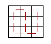
A grid is a special form of a graph with the formal term lattice, where any node have edges to its neighbours determined by the location within the grid. There are more graph types like multi-graphs, with multiple edges between the same nodes.

Simply put, a graph is a collection of nodes with edges connecting the nodes together in different ways.

In map programs and satellite navigation systems, edges can be assigned a cost which correlates to some euclidean distance of the edge, or road surface type in real world applications. The cost is typically the geometrical distance between cities. Other cost factors can be what type of road it is, a highway, country road, gravel road or a donkey path. A highway has a lower cost than a donkey path, which is honoured by the algorithm working its way through possible paths.

A cost based path finding algorithm works its way through a graph by searching for the most efficient (lowest cost) path based on edge costs and heuristic values. Let's see how this works.

Algorithms

There are many algorithms for navigating graphs and these are perhaps the most common ones:

• Breadth First Search explores equally in all directions. It's a useful algorithm for map analysis and it will always find the shortest path, but it's also time consuming by exploring all possible paths.
• Depth First Search explores in one direction, at first. When it reaches a dead-end it steps back and attempts another path until finding the destination. It's a useful algorithm for tree traversals and maze solving, but it doesn't necessarily find the shortest path.
• Dijkstra’s Algorithm works by prioritising which paths to explore. Instead of exploring all possible paths equally, it favours lower cost paths. For that reason it's also called a uniform cost search. You can assign lower costs to encourage moving on roads, higher costs to avoid forests or hills, even higher costs to avoid going near enemy fortifications, and more. It's most useful when movement costs varies a lot.
• A* Search is a modification of Dijkstra’s Algorithm that is optimised for a single goal/destination. Dijkstra’s Algorithm can find paths to all locations. A* finds paths to one specific location. It prioritises paths that seem to be leading closer to a goal based on a heuristic or estimate. A* is a common algorithm for path finding in games because it combines the strengths of both breadth first and Dijkstra's.
• Bellman-Ford Algorithm is a special shortest path algorithm targeted for graphs with negative edge costs. It solves the same problem as Dijkstra's but with a non-greedy approach. It's less efficient but more versatile and can be used for graphs with negative edge cost where other algorithms won't work. It's useful for network flow analysis where something flows through a network of nodes (traffic, electricity, water, air, etc).

The idea behind these algorithms is to track an expanding ring around the start node called the frontier or fringe. The real difference lies in how this ring expands as part of finding the optimal path.

Let's explore these algorithms more but focus on the cost-based algorithms Dijkstra's and A* .

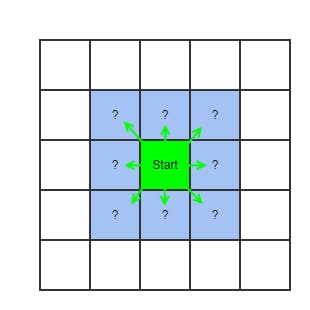
Breadth First Search (BFS)

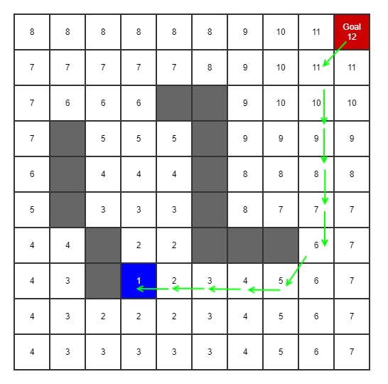
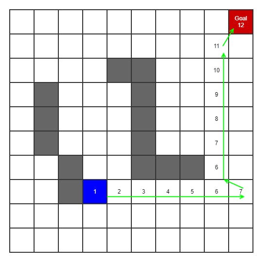
BFS starts by marking the current or starting node as 1. Then it expands to all adjacent nodes, marking these as 2. Then all adjacent nodes to them as 3, etc, until the target node is found. It then counts backwards by one:s to the start node and out of that comes the shortest path when inverted.

Breath first is always guaranteed to find the shortest path, if there is a path. However, as a greedy algorithm it visits all possible nodes in the graph to find the best path, making it potentially slow.

Depth First Search (DFS)

DFS is similar to BFS. It starts by marking the current or starting node as 1. Then it expands to one adjacent nodes by random, marking that as 2. Then it continues to next adjacent nodes in the same vector until a dead end is reached. It then returns the last node which was a junction and tries in that direction. This continues until the target node is found. It then counts backwards by 1:s to the start node and out of that comes the shortest path.

Depth first is not guaranteed to find the shortest path, but its generally faster by not having to search all possible nodes in the graph.

Dijkstra's

Dijkstra's is an algorithm invented by Edsger W. Dijkstra in 1956 and it constitutes the foundation for most cost-based, shortest-path finding algorithms to this day.

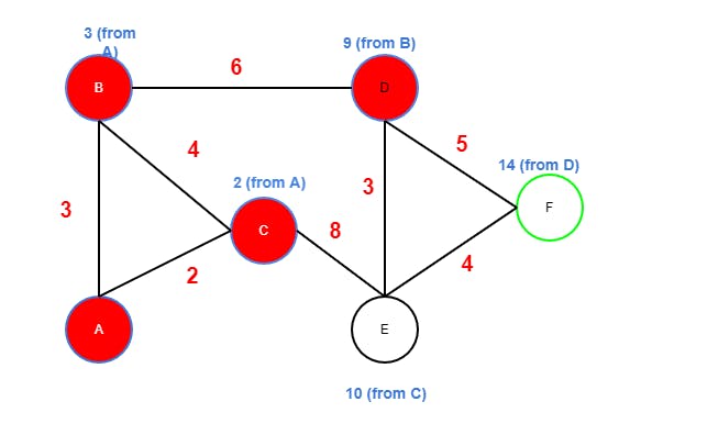
Imagine the graph below with six nodes labeled A to F. The starting node is A (blue) and target node is F (green). The edge costs (in red) are predetermined and will not change.

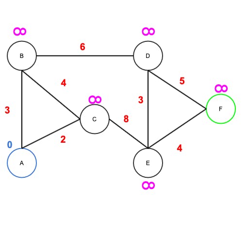
We wan't to find the shortest path between these nodes, which correlates to the lowest cost path.

Dijkstra's Solution

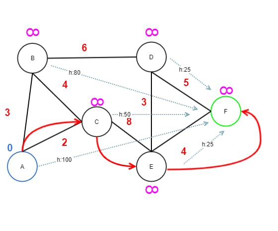
1. Initially, all node costs (above the rings) are set to INF, except for the starting node A which has cost 0 since it's the starting node.
2. All nodes are marked as unvisited.
3. For the current node, follow the edges to nearest unvisited neighbours, calculate the temporal edge cost and add it to the current node cost. Initially:

   a) A to A → 0
   b) A to C →  0 + 2 = 2
   c) A to B →  0 + 3 = 3
   

4. Compare the temporal value against all unvisited neighbours, and update each node if the value is less than the currently calculated cost.

   a) A to C →  2 which is less than INF, so set to 2
   b) A to B →  3 which is less than INF, so set to 3
   

5. When all unvisited neighbours are visited and calculated, mark the current node as visited. It will never be visited again.
6. If the target node has been visited, the algorithm is complete. Shortest path found and early exit is possible!
7. If not, move on to the next unvisited neighbour with the lowest edge cost and repeat from step 3.

Next, a step-by-step breakdown of how the algorithm works for the same example graph.

Detailed Steps

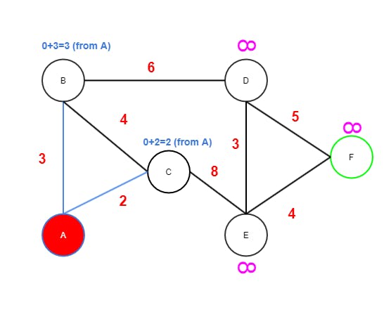
Step One

1. The start node A has edges to B and C.
2. B gets value 3 from A because 3 is less than INF. The from (or parent node) reference is important. It's used later as a breadcrumb to resolve the path backwards.
3. C gets value 2 from A since 2 is less than INF.
4. A is marked as visited (red).
5. C now has the lowest tentative value 2 of currently unvisited nodes and therefore becomes the next node to continue from.

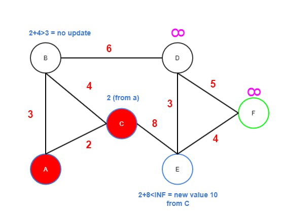
Step Two

1. C is now the current node and it has edges to B and E.
2. B has value 3, so its new value would be 6 (2+4) which is higher than 3, so B is not updated.
3. E has value INF which is higher than 10, so E is updated to 10 (from C).
4. C is marked as visited and will never be visited again.
5. B has the lowest tentative value 3 (over 10 of E) of currently unvisited nodes, and therefore becomes the next node.

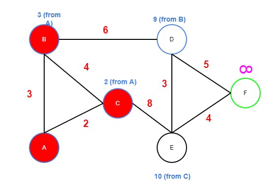
Step Three

1. B is now the current node and it has only one edge to D since A and C are marked as visisted.
2. 3+6 is less than INF (it has to be), so update D to 9 and mark B as visited.
3. D will become the next node.

Step Four

1. D is now the current node and it has edges to F and E that are unvisited.
2. 9+5 is less than INF so update F to 14 from D.
3. Target node F was visited so the algorithm is now complete, but let's finish the run!
4. 9+3 is higher than 10 so skip E.
5. Mark D as visited.

Resolution

The shortest path is resolved by following the breadcrumbs (back tracking) from the target node F.

F → D = 5
D → B = 6
B → A = 3

By inverting the path we finally get the shortest path from start node A:

 A -> B -> D -> F

Total travel cost is 14. Worth noticing is that A→ C → E → F gives the same total cost (14) so there are two equally fast paths in this graph.

A* Search

The A* search algorithm is a generalised form of Dijkstra's with a heuristic factor (H-cost) that makes it more efficient.

This algorithm requires less compute cycles when considering alternative paths by adding a heuristic cost to the node cost. This is in fact the only thing that separates it from Dijkstra's. A heuristic cost added to node movement (G) costs makes the algorithm gravitate towards the destination node.

The important thing to notice is that the heuristic must never be overestimated. If it is, the algorithm will fail to find the shortest path and instead it will find some path, if one exists. The heuristic must always be less or equal to the actual cost for the A* algorithm to find the shortest path.

One approach is to use the euclidean distance of each node to the target node as the heuristic cost factor. The algorithm works exactly the same way as Dijkstra's by estimating neighbouring nodes lowest cost, called the f cost.

If we first look at Dijkstra's, its:

f cost = g cost
g cost = distance from starting node

The A* algorithm only adds a heuristic called h, which is a the estimated cost to the end node from each visited node:

f cost = g cost + h cost
g cost = distance from starting node
h cost = distance to end node (heuristic)

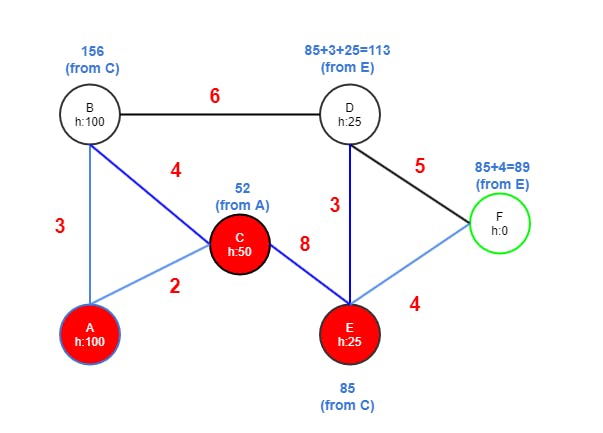
By assuming the same diagram below with nodes A to F and a heuristic estimate of the euclidean distance from each node to node F. The h cost for F is zero.

What would be the shortest path? Answer is A→ C→ E → F. The reason is that while the path cost (14) is the same as for A → B→ D → F, in this case the heuristic makes it more expensive to go via B. You can even swap the edge weights of A→ B and A→ C and the shortest path is still the same, via B. If you drag B almost to the same distance as C from F, then the path will change to B.

Let's do a step-by-step breakdown of how the algorithm works.

Detailed Steps

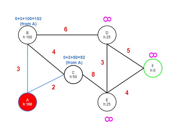
Step One

• A has edges to B and C.
• B gets value 3 from A because 3 is less than INF. Then the heuristic estimate of 100 is added, with a total of 103. This becomes B's f cost. → (103) f cost = (3) g cost + (100) h cost
• C gets vale 2 from A since 2 is less than INF, adding 50 with a total of 52.
• A is marked as visited (red).
• C now has the lowest tentative value 52 of currently unvisited nodes and therefore becomes the next node to continue from.

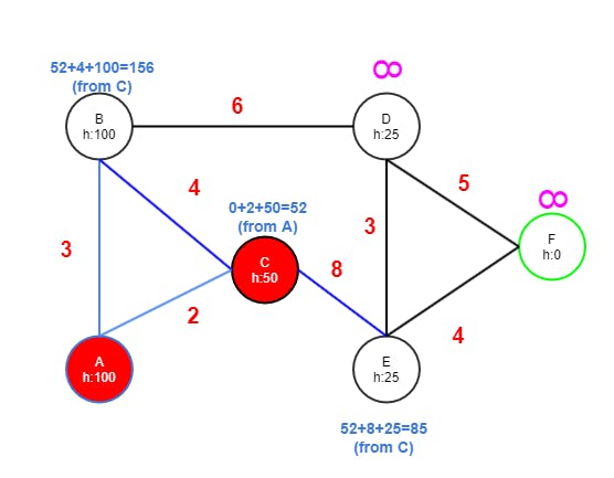
Step Two

• C has edges to B and E.
• B gets value 52+4 from C because it's less than 103. Adding the h cost of B (100) results in 156.
• E gets value 52+8 from C because it's less than INF. Adding the h cost of E (25) results in 85.
• C is marked as visited (red).
• E now has the lowest tentative value 85 of currently unvisited nodes and therefore becomes the next node.

Step Three

• E has edges to D and F.
• D gets value 85+3 from E because it's less than INF. Adding the hcost of D (25) results in 113.
• F gets value 85+4 from E because it's less than INF. The h cost of F is zero since its the goal node resulting in 89.

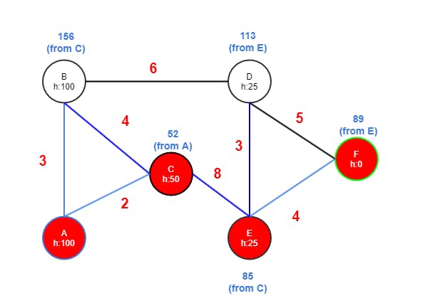
Step Four

The A* algorithm is now completed and the shortest path to the goal node is found. It could exit here or continue examining D and B. However, it's of no good since a shorter path will not be discovered.

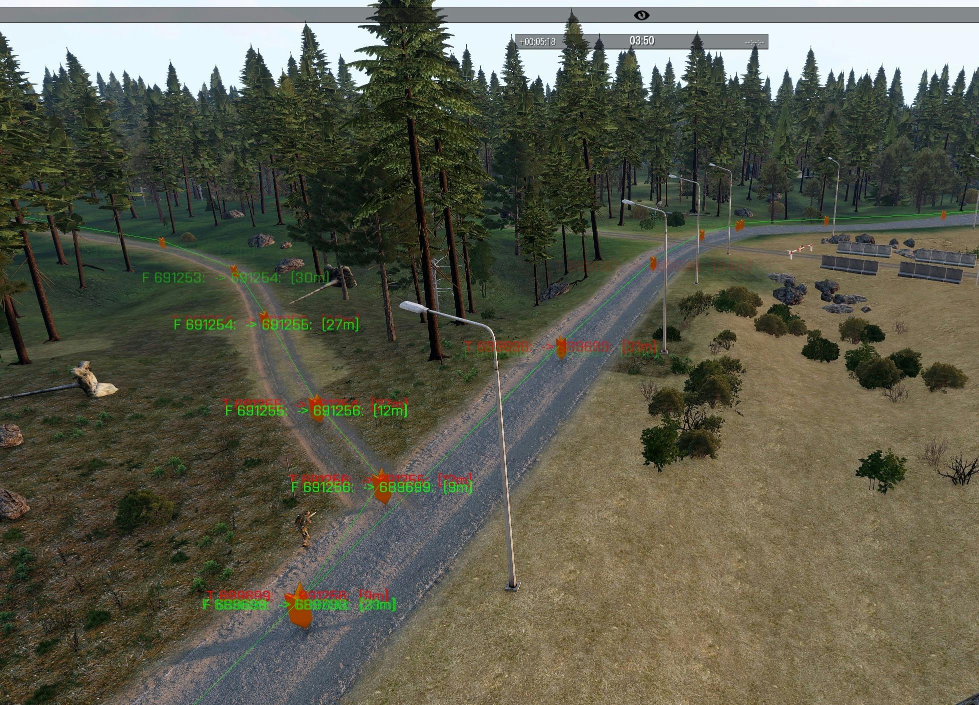
Game Example

Example of path finding using A* search on a map grid. In the map below, each green circle is a highlighted road segment which are basically nodes in a graph. The algorithm starts by walking through all discoverable road segments in a breadth first search. After that's done, A* takes over and works its way through all nodes. It uses the euclidean distance of each node to the goal node as H cost value. It's simple to do in this particular game through a 2D distance function between two positions.

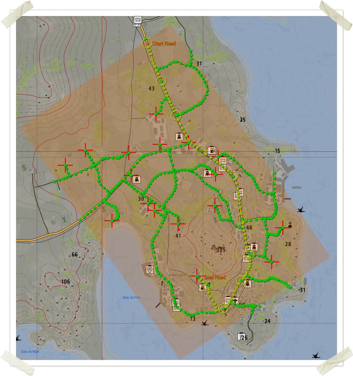
A recorded demo is available in Github

Dijkstras in Arma Script

The demo above uses this implementation (in Arma script):

#include "script_component.hpp"
/*
    Author: Kai Niemi
    Dijkstra's algorithm to find shortest path between two vertexes in a graph (network of roads).
    Arguments:
    0: start vertex/road <OBJECT>
    1: goal vertex/road <OBJECT>
    2: generated graph edges (road map) <ARRAY>
    Return Value:
    predecessors to all vertexes in the graph, i.e. shortest distance to each node in
    the graph from the start node.
    Public: No
*/
params[
    ["_startNode", objNull, [objNull]],
    ["_endNode", objNull, [objNull]],
    ["_edges", [], [[]]]
];

if (isNull _startNode) exitWith { ERROR("Start node is required!"); [] };
if (isNull _endNode) exitWith { ERROR("End node is required!"); [] };

DEBUG_1("Applying Dijkstra's Algorithm on %1 edges", count _edges);

private _predecessorList = [];
private _visitedList = [];
private _unvisitedList = [];

// Create hash table for node distances
private _distanceHash = [[[_startNode, 0]], POSITIVE_INFINITY] call CBA_fnc_hashCreate;
private _predecessorHash = [[], -1] call CBA_fnc_hashCreate;

_unvisitedList pushBack _startNode;

private _startTime = diag_tickTime;
private _iterations = 0;

// Loop until unvisited priority queue is empty
while {count _unvisitedList > 0} do {
    // Find unvisited node with smallest known distance from the start node.
    private _current = [_distanceHash, _unvisitedList] call FUNC(unvisitedLowestCost);
    if (_current isEqualTo _endNode) exitWith {
        INFO_1("Found end node %1", _endNode);
    };

    // Remove vertex from unvisited set
    _unvisitedList deleteAt (_unvisitedList find _current);

    // Add current node to visited set
    _visitedList pushBackUnique _current;

    // Distance to current node
    private _currentDist = [_distanceHash, _current] call CBA_fnc_hashGet;

    // Find all unvisited neighbors
    private _unvisitedNeighbors = [_edges, _visitedList, _current] call FUNC(unvisitedNeighbors);

    // For the current node, calculate the weight of each neighbor from the source node
    {
        private _neighbor = _x;

        private _edgeWeight = [_edges, _current, _neighbor] call FUNC(edgeWeight);

        private _totalDist = _currentDist + _edgeWeight;

        private _tentativeDist = [_distanceHash, _neighbor] call CBA_fnc_hashGet;

        // Update neighbour if distance is less
        if (_totalDist < _tentativeDist) then {
            [_distanceHash, _neighbor, _totalDist] call CBA_fnc_hashSet;

            // Store predecessor from where this neighbour was visited
            private _idx = [_predecessorHash, _neighbor] call CBA_fnc_hashGet;
            if (_idx >= 0) then {
                _predecessorList set [_idx, [_neighbor, _current]];
            } else {
                _idx = _predecessorList pushBack [_neighbor, _current];
                [_predecessorHash, _neighbor, _idx] call CBA_fnc_hashSet;
            };

            // Add neighbour to unvisited set to reset
            _unvisitedList pushBackUnique _neighbor;
        };
    } foreach _unvisitedNeighbors;

    _iterations = _iterations + 1;
};

DEBUG_3("Dijkstra's algorithm done in %1s - found %2 predecessors in %3 iterations",
    diag_tickTime - _startTime, count _predecessorList, _iterations);

_predecessorList

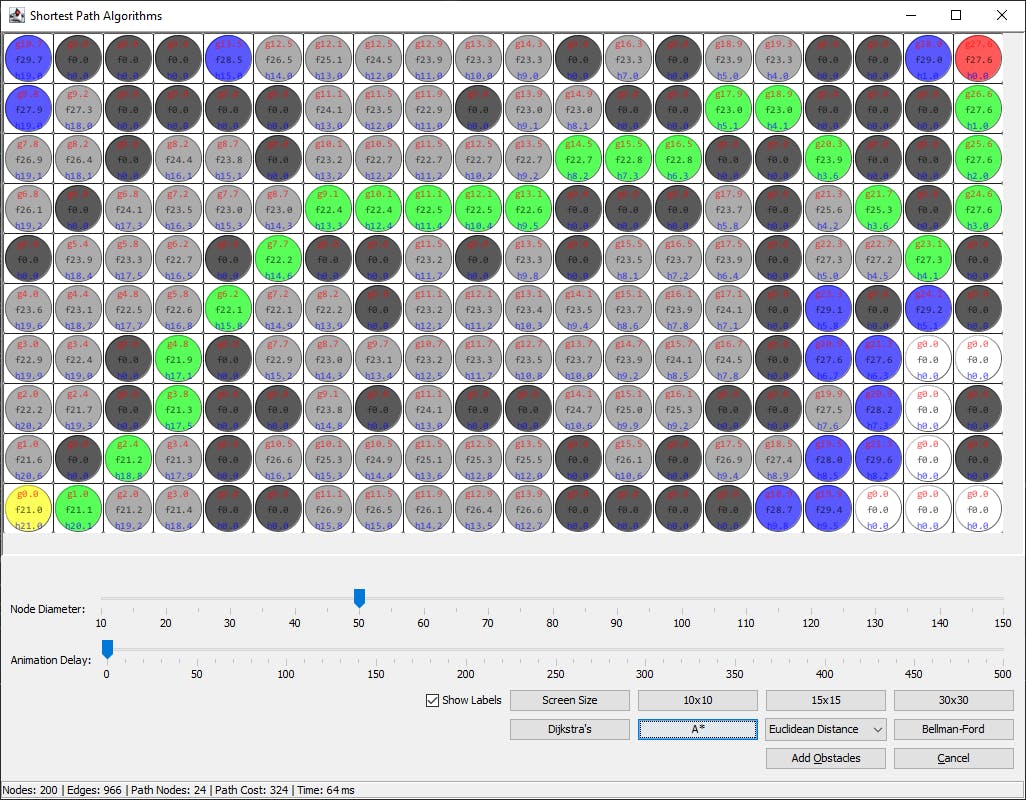
Java Application

Below is a java client application visualising how the search algorithms work.

Dijkstras in Java

Search implementation using Dijkstras:

public class DijkstrasAlgorithm<N> implements SearchAlgorithm<N> {
    private FringeListener<N> fringeListener = new EmptyFringeListener();

    private final TraversableGraph<N> graph;

    public DijkstrasAlgorithm(TraversableGraph<N> graph) {
        this.graph = graph;
    }

    public void addFringeListener(FringeListener<N> fringeListener) {
        this.fringeListener = fringeListener;
    }

    @Override
    public List<N> findShortestPath(N start, N goal) {
        // Set initial cost to infinity and clear path
        for (Node<N> node : graph.nodes()) {
            node.setG(Double.MAX_VALUE);
            node.setH(Double.MAX_VALUE);
            node.setParent(null);
        }

        final Node<N> goalNode = graph.wrap(goal);

        // Distance from source to source is set to 0
        final Node<N> startNode = graph.wrap(start);
        startNode.setG(0);
        startNode.setH(heuristicCostEstimate(startNode, goalNode));

        // Add source vertex to unvisited set, aka fringe or frontier
        Queue<Node<N>> openSet = new PriorityQueue<>(Comparator.comparingDouble(Node::getF));
        openSet.add(startNode);

        fringeListener.nodeVisited(startNode);

        // Holds all visited/settled vertexes
        Set<Node<N>> closedSet = new HashSet<>();

        while (!openSet.isEmpty()) {
            // Find unvisited vertex with smallest known distance from the source vertex.
            // This is initially the source vertex with distance 0.
            Node<N> currentNode = openSet.poll();

            // Early exit
            if (currentNode.equals(goalNode)) {
                break;
            }

            // Add vertex to visited set
            openSet.remove(currentNode);
            closedSet.add(currentNode);

            fringeListener.nodeClosed(currentNode);

            // For the current vertex, calculate the total weight/cost of each neighbor from the source vertex
            for (Node<N> neighborNode : unvisitedNeighbors(currentNode, closedSet)) {
                // Grab edge cost and add it to the movement or G-cost of current node
                double edgeCost = graph.edgeValue(currentNode, neighborNode).get();

                double tentativeCost = currentNode.getG() + edgeCost;

                if (tentativeCost < neighborNode.getG()) {
                    neighborNode.setParent(currentNode);
                    neighborNode.setG(tentativeCost);
                    neighborNode.setH(heuristicCostEstimate(neighborNode, goalNode));

                    openSet.add(neighborNode);

                    fringeListener.nodeVisited(neighborNode);
                }
            }

            if (fringeListener.simulationDelay() > 0) {
                try {
                    Thread.sleep(fringeListener.simulationDelay());
                } catch (InterruptedException e) {
                    Thread.currentThread().interrupt();
                }
            }
        }

        // Backtrack and we have the path
        List<N> trail = new ArrayList<>();
        trail.add(goalNode.getValue());

        Node<N> parent = goalNode.getParent();
        while (parent != null) {
            trail.add(parent.getValue());
            parent = parent.getParent();
        }

        Collections.reverse(trail);

        return trail;
    }

    protected double heuristicCostEstimate(Node<N> from, Node<N> goal) {
        // Always zero in Dijkstra's, its only thing what separates it from A*
        return 0;
    }

    private Set<Node<N>> unvisitedNeighbors(Node<N> node, Set<Node<N>> visited) {
        Set<Node<N>> neighbours = new HashSet<>();

        graph.adjacentNodes(node, end -> {
            if (!visited.contains(end)) {
                neighbours.add(end);
            }
        });

        return neighbours;
    }
}

A-* in Java

Turning Dijkstras to A-star is all about the h-cost as mentioned in this article:

public class AStarAlgorithm<N> extends DijkstrasAlgorithm<N> {
    private final HeuristicCost<N> heuristicCost;

    public AStarAlgorithm(TraversableGraph<N> graph, HeuristicCost<N> heuristicCost) {
        super(graph);
        this.heuristicCost = heuristicCost;
    }

    @Override
    protected double heuristicCostEstimate(Node<N> from, Node<N> goal) {
        return heuristicCost.estimateCost(from.getValue(), goal.getValue());
    }
}

The cost function has three variants:

• Diagonal Octile Distance
• Euclidean Distance
• Manhattan Distance

Conclusions

In this article we explored a few common shortest path search algorithms that are used all around us. These algorithms share a common goal which is to find the lowest-cost path between two points in a graph. They mainly differ in how the ring or fringe expands when exploring alternative paths.